[BA03. Bayesian On-Time Risk: App 1] Anatomy of the EXA Engine: Mixture Distribution and Observation Deviation

This article is the first in a technical commentary series clarifying the operating principles of the EXA engine featured in the novel-format serialized episode ‘BA03 On-Time Material Inbound: Bayesian MCMC‘.

This series deals with Mixture Distribution and MCMC (Markov Chain Monte Carlo) Gibbs Sampling, which belong to advanced techniques among Bayesian inference, so the content may be deep and the calculation process somewhat complex. Therefore, to make this as digestible as possible, we intend to approach it in detail by dividing it into stages, and it is expected to be a rather long journey.

For a full understanding of the context, we recommend reading the original episode first. Additionally, since Bayesian theory expands concepts step-by-step, reviewing the episodes and mathematical explanations of BA01 and BA02 first will be much more helpful in accepting this content. This is because the preceding mathematical concepts and logic continue here.

1. Definition of Data: Observation Deviation

To mathematically model ‘On-Time’, the key issue dealt with in the novel, we must first define the data. To this end, we generate sample observation data in Day units as follows:

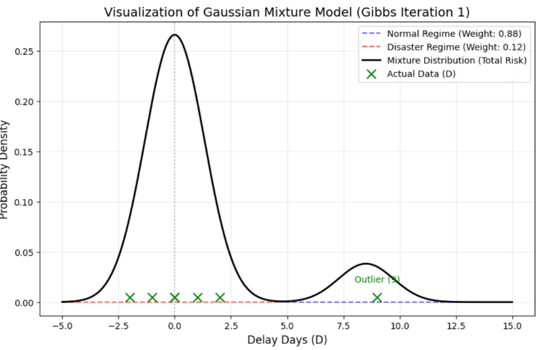
$$D = [d_1, d_2, \dots, d_7] = \{ -2, -1, 0, 1, 2, 0, 9 \}$$

We can view this set of observed delay days, $D$, as a single Vector, and each delay value (-2, -1, 0 …) included therein becomes an Element (or component) constituting this vector.

Here, the individual data element $d_i$ is defined as follows:

$$d_i = (\text{Actual Date}) – (\text{Planned Date})$$

The meaning of this formula is very intuitive.

• $d_i = 0$: When the promise is kept exactly (On-Time)
• $d_i > 0$: When delayed compared to the plan (e.g., +5 means 5 days delay)
• $d_i < 0$: When arrived earlier than planned (Early Inbound)

This Delay Days model can be applied to measure various Bottlenecks in business sites.

• Material inbound and supplier’s work delay (Lead Time Delay)
• Transportation and logistics delay (Transportation Delay)
• Process delay in production lines (Production Delay)

The size (dimension) of the vector data is determined by the business scale. If there are 100 observed transaction records, it will be a vector composed of 100 elements; if 300 records, it will be a vector composed of 300 elements.

In this series, to clearly dissect the operating principles of the EXA engine, we use the 7 pieces of ‘Toy Data’ defined above as an example. While hundreds or thousands of data points are realistic, there are limits to intuitively showing complex calculation processes with them.

Of course, when applied to actual sites, data must be managed by segmenting (Granularity) according to decision-making purposes, such as “Supplier + Item + Transportation Mode + Destination” or “Line + Product” for production, and through this, risks across the entire SCM can be accurately captured.

2. Visualization of Data: Two Peaks

Now, let’s visualize our Toy Data (Vector $D$). Let’s check how the 7 elements are distributed on the graph.

What about real-world data? Below is a histogram representing 200 actual material purchase transaction records (specific item from a specific supplier) of a certain company.

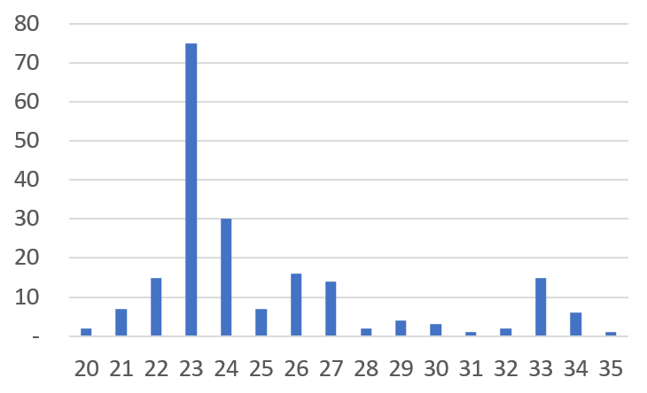
An interesting similarity is discovered. Our Toy Data is scattered around the Normal State (0) while simultaneously forming a separate peak called the Delay State (9). The actual company data is also divided into a peak centered around the average of 23 days, which is the normal lead time, and another (albeit weaker) peak centered around 33 days, which is the delay state.

Most Delay Days data take on a form with two peaks like this. In actual data, three or more peaks may sometimes appear. However, rather than modeling every peak of the data individually, we compress it into a 2-Regime (Normal/Delay) structure to match the structure in which decision-making is actually executed (Normal Operation vs. Abnormal Response).

This is not simply to shrink reality. It is an aspect of Operational Design to reduce uncertainty, stabilize judgment, and make execution consistent. Detailed patterns (such as minor delays) can be expanded when necessary, but the basic engine is most robust when defined by two states (Regime): ‘Normal’ and ‘Delay’.

3. Statistical Assumption: Validity of Normal Distribution

Here, we establish one important statistical assumption. “Delay Days data follows a Normal Distribution scattered in a bell shape around the mean.”

Why specifically the Normal Distribution?

Some might ask, “Does reality truly follow the Normal Distribution like a textbook?” However, according to the Central Limit Theorem in statistics, the result value that appears when various independent variables (worker’s condition, weather, traffic situation, minute machine errors, etc.) are combined converges to a Normal Distribution if the sample is sufficient. In other words, modeling the uncertainty of processes and logistics with a Normal Distribution becomes the most mathematically valid and rational approach.

4. Conclusion and Next Steps

Ultimately, this graph we are looking at is a combined form of the ‘Normal Distribution of the Normal State’ and the ‘Normal Distribution of the Delay State’. This is the reality of the Mixture Distribution that the EXA engine in the novel intends to interpret.

[Conclusion of Part 1] The data we observed, that is, the Likelihood function, is a Mixture Distribution where two individual Normal Distributions are mixed.

The primary goal is to find the On-Time Risk, that is, the probability that a delay can occur, from the observation data composed of this Mixture Distribution using Bayesian Inference.

To this end, in the next article [Appendix 2], we will design a concrete mathematical model to solve the Likelihood function composed of the Mixture Distribution using Bayesian methods.