Decision Impedance Matching

Through the previous Part 1 and Part 2 of the BA02 [Exa Bayesian Inference] “The Invisible Hand of Sales: A 60-Day Gamble” episode, we explored how the Bayesian Engine establishes ‘Prior Beliefs’ and tracks the trajectory of probability through ‘Signals’ and ‘Silence’. Now, we hold in our hands the pure posterior probability, P_raw meticulously calculated by the Bayesian parameters α and β.

But it is not over yet. The final decision-making process remains. Even with a probability of 60%, the weight of the decision can vary completely depending on whether it was obtained from a single meeting or derived after dozens of negotiations.

Unfortunately, the human brain does not operate on linear numbers alone. In today’s Appendix Part 3, we explore the secret of ‘Decision Impedance Matching’, which transforms cold probability into the language of decision-making through the ‘total amount of evidence’ held by Bayesian parameters.

1. The Swamp of Numbers: Why is 51% Insufficient for a Decision?

Mathematically, 51% is over half, so it implies a ‘high possibility of success’. However, in the life-or-death field of business, 51% is practically no different from an ‘all-or-nothing’ gamble.

The most dangerous thing in the business field is ‘groundless optimism’.

• Situation A: α=0.6, β=0.4 (P=60%)
• Situation B: α=60, β=40 (P=60%)

The mathematical probability (P) is 60% for both. However, from a leader’s perspective, Situation A is a ‘gamble left to luck’, while Situation B is a result of numerous verifications (The sizes of α and β in A and B are different. In other words, the magnitude of belief is different). The former is an unstable state that can swing to 0% or 100% with the slightest breeze, whereas the latter is a state with ‘inertia’ that does not waver easily even with bad news.

The human brain does not simply look at the ‘ratio’. It intuitively calculates the ‘thickness of evidence’ underlying it. We need to explicitly specify this intuition into the system’s logic.

Humans detest uncertainty and have a nature to reserve action until a certain ‘Threshold’ is crossed. Conversely, once convinced, they accept 85% probability or 95% probability equally as ‘certainty’.

Thus, a huge gap exists between ‘mathematical probability’ and ‘psychological conviction’. Just as ‘impedance matching’ is done in electronics to reduce energy loss when connecting two different circuits, a sophisticated tuning connecting the system’s numbers and human decisiveness is required.

2. Total Amount of Evidence (n): Critical Mass of Decision Making

The Exa engine applied in the BA02 episode uses the Bayesian posterior probability (expressed here as P_raw) and the total amount of evidence (n = α + β) as a filter for decision-making. This is the core of ‘Decision Impedance Matching’.

2.1 Volume of Trust and Information Density

The Bayesian parameters α and β are the accumulated weights of ‘evidence of success’ and ‘evidence of failure’, respectively. The sum of the two, n, becomes an indicator representing ‘how much we know’ about this deal.

• When n is small (Energy Mismatch): No matter how high the system’s probability is, it does not lead to the leader’s conviction. Because it is risky. This is a state where energy is not transferred because the circuit impedance does not match. At this time, the engine sends a warning of “Not Enough Evidence” instead of probability.
• When n is large (Impedance Matching): The probability number begins to resonate with the leader’s decisiveness. Since sufficient evidence has accumulated, a 1% change in probability is now precisely transmitted as a 1% change in actual business risk.

Accordingly, the engine captures the organization’s accumulated total knowledge and reshapes the number by passing it through a ‘Sigmoid Function’ similar to the human cognitive structure.

2.2 Sigmoid Calibration: Embedding ‘Will’ into Probability

We adjust the density of probability through the following non-linearity.

$$P_{calibrated} = \frac{1}{1 + e^{-k(P_{raw} – P_{0})}}$$

Here, P_raw is the source Bayesian posterior probability calculated by the engine, k is the slope of conviction (strength of conviction), and P₀ is the decision-making threshold.

• Gentle Zone (Uncertainty): When the probability is between 30-50%, the calibrated value moves very conservatively. It is a signal saying “Don’t trust it yet.”
• Steep Zone (Decision): The moment the probability exceeds 60%, the sigmoid curve rises steeply. A single small positive signal raises the probability from 60% to 80%.
• Saturation Zone (Conviction): Once it exceeds 85%, the curve becomes gentle again. It reflects that 90% or 95% is the same ‘Commit’ state for humans.

From now on, let’s overview the key concept Log-odds used in decision impedance matching, dig into the inside of the engine mathematically, and finally understand this through a business simulation.

3. The Hidden World: Accumulation of Log-odds

Looking inside the engine where Exa’s Bayesian update occurs, probability does not look like the 0-100% we know. Bayesian parameters α, β mathematically operate in an infinite linear space called ‘Log-odds’.

$$logit(P) = \ln\left(\frac{P}{1-P}\right) = \ln\left(\frac{\alpha}{\beta}\right)$$

Every time we get a new signal in the sales meeting process, the system honestly adds this Log-odds value.

• Success signals captured during negotiation push the value up via +Δα.
• Failure signals and time decay (λ) pull the value down via +Δβ.

This process is like the accumulation of charge in an electric circuit. However, this energy is still only ‘voltage inside the circuit’, and to convert it into ‘power’ that runs actual devices, an interface that meshes with external resistance is needed.

3.1 Mapping to Sigmoid Probability

Why specifically the Sigmoid function? Because Sigmoid is the Inverse Function of the Log-odds function above. It is the only mathematical solution that returns the sum of evidence accumulated in an infinite range (-∞ ~ +∞) to the probability world between 0.0 and 1.0 that we can understand.

$$P = \frac{1}{1 + e^{-k(x – x_0)}}$$

Here, x is the Log-odds ($ln\frac{α}{β}$) we have accumulated. This formula is not simply a device to make numbers pretty, but a device to compress the energy of infinite information into a finite range of decision-making.

3.2 World of Probability vs. World of Information

The world we live in converses in ‘Probability’, but the principle by which data accumulates is ‘Information Accumulation’.

• World of Probability (0 ~ 1): This world is very narrow and stifling. It is hard to go from 0.9 to 0.99, and it is blocked by the wall of 1.0. Adding or subtracting numbers here hits a wall quickly. (e.g., 0.9 + 0.2 = 1.1 → Impossible)
• World of Information (-∞ ~ +∞): This world is endless. As evidence accumulates, the number can become infinitely large, and if contrary evidence appears, it can become infinitely small.

Log-odds is a map that unfolds this narrow world of probability into a vast world of information.

3.3 Why Log-odds is More Reasonable and Persuasive

① ‘Additivity’ of Evidence

The core of Bayesian update is modifying probability whenever new information comes in. In probability space, complex multiplication and division must be repeated for this, but in Log-odds space, it becomes simple addition.

“Today’s meeting was good (+2 points), but a competitor appeared (-1.5 points).”

The reason we can intuitively score and add like this is that our brain is already internally performing linear calculations similar to Log-odds.

② Removal of the ‘Walls’ of 0 and 1

When the probability is 99.9% and 99.99999%, we feel both are “almost certain,” but a huge amount of additional evidence is needed between them. Log-odds accurately portrays the business truth that “the deeper the conviction, the more evidence is needed” by expanding the numbers geometrically as they approach 1.

③ Symmetry

A situation with 80% success probability and a situation with 80% failure probability (20% success) are like two sides of a coin. In Log-odds space, these two situations appear as +1.38 and -1.38. In other words, positive and negative energies form perfect symmetry like a mirror, ensuring logical consistency.

3.4 Connection with Bayesian Parameters

Expressing Log-odds (L) using α and β is as follows:

$$L = \ln\left(\frac{\alpha}{\beta}\right)$$

• If success evidence (α) increases, L becomes large positive (+).
• If failure evidence (β) increases, L becomes small negative (-).
• If the weights of both are equal, L becomes 0. (Probability 50%)

Like this, Log-odds is like the scale of a balance that determines “Whose voice is louder?” This is the big picture of why Log-odds is a concept that ‘unfolds probability into infinite information space for linear calculation’ and becomes a “more reasonable basis” in business logic.

4. Mathematical Development

For readers who are more curious, I intend to show step-by-step how Bayesian parameters (α, β) in Exa’s engine pass through the passage of Log-odds and settle into the exponent part of the Sigmoid function. Depending on the reader, this part might be the most interesting time.

4.1 Starting Point: Bayesian Posterior Probability (P)

First, we define the pure probability P calculated using our updated protagonists α and β.

$$P = \frac{\alpha}{\alpha + \beta}$$

This P value moves between 0 and 1, and is the (posterior) probability, i.e., win rate, that we intuitively understand.

4.2 Conversion to Log-odds

Now, unfold this probability into Log-odds (x), an infinite information space. Developing the formula according to the definition of Log-odds yields a surprising result.

$$x = \ln\left(\frac{P}{1-P}\right)$$

Let’s substitute the P value defined above into this.

$$x = \ln\left(\frac{\frac{\alpha}{\alpha + \beta}}{1 – \frac{\alpha}{\alpha + \beta}}\right) = \ln\left(\frac{\frac{\alpha}{\alpha + \beta}}{\frac{\beta}{\alpha + \beta}}\right) = \ln\left(\frac{\alpha}{\beta}\right)$$

In other words, Log-odds x simply becomes the value obtained by taking the log of the ratio of success evidence (α) and failure evidence (β). This is the ‘weight of pure evidence’ we have accumulated in the world of information.

4.3 Conversion of Decision Threshold (T)

The decision threshold T is also a probability unit (e.g., 0.8). Convert this to x₀, the reference point in Log-odds space.

$$x_0 = \ln\left(\frac{T}{1-T}\right)$$

Now we are ready to compare all data on the same scale called ‘Log-odds’.

4.4 Final Sigmoid Combination (Impedance Matching)

Now, finally, put all these values into the exponent part of the Sigmoid function. The Sigmoid function accepts the ‘difference between current energy (x) and reference energy (x₀)’ in its exponent part.

$$P_{out} = \frac{1}{1 + e^{-k(x – x_0)}}$$

Let’s substitute x and x₀ obtained above into this equation and organize the exponent part.

$$-k \left( \ln\frac{\alpha}{\beta} – \ln\frac{T}{1-T} \right) = -k \ln\left( \frac{\alpha / \beta}{T / (1-T)} \right)$$

Therefore, the final formula transforms as follows:

$$P_{out} = \frac{1}{1 + \left( \frac{\beta \cdot T}{\alpha(1-T)} \right)^k}$$

4.5 Mathematical Conclusion and Business Meaning

Let’s summarize why this development proves ‘critical mass’ and ‘persuasiveness’.

1. Magic of Exponent: As the complex e and ln in the exponent part meet and cancel each other out, only the relative magnitude of the success ratio ($\frac{α}{β}$) and the target ratio ($\frac{T}{(1-T)}$) remains as a result.
2. Power of k: As k is located in the exponent position, even if the success evidence slightly exceeds the target, it increases the probability steeply.
3. Reflection of Data Weight: It does not simply look at probability (P), but as the absolute amount of evidence called α and β increases, the power of this ratio becomes more solid.

5. Business Simulation

Let’s prove how this mathematical model creates ‘Energy of Decision’ through an actual business scenario.

Assume we set the master reference values according to the tendency of an organization as follows.

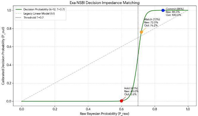
• Decision Threshold (T): 0.7 (70%)
  • Interpretation: “There must be at least 70% probabilistic basis to be worth a try.”
• Decision Acceleration (k): 10
  • Interpretation: “Once the threshold is crossed, act aggressively.”
• Final Formula:$$P_{out} = \frac{1}{1 + \left( \frac{\beta \cdot T}{\alpha(1-T)} \right)^k}$$

5.1 Simulation Business Scenario

Now, consider a stage in the sales negotiation process where the initial belief (prior distribution) has a sequentially updated posterior distribution. The α and β below are values updated in the Bayesian engine from the Stage and Signal of the negotiation process so far.

Situation 1: Below Threshold (Uncertain State)

• Data: α=6.0, β=4.0 (Pure Probability P_raw = 60%)
• Calculation Process:
  • Ratio Calculation: $\frac{(4.0 * 0.7)}{(6.0 * 0.3)}$ ≈ 1.55
  • Applying power of k: $1.55^{10}$ ≈ 81.3
  • Final: $P_{out}$ =$\frac{1}{(1 + 81.3)}$ ≈ 1.2%
• Interpretation: Bayesian probability is 60%, but it falls short of the organization’s standard $P_{out}$ (70%). The system blocks the decision energy and sends a suppression signal of “Don’t trust it yet absolutely (Hold)” to the decision-maker.

Situation 2: Threshold Breakthrough (Start of Decision)

• Data: α=7.2, β=2.8 (Pure Probability $P_{out}$ = 72%)
• Calculation Process:
  • Ratio Calculation: $\frac{(2.8 * 0.7)}{(7.2 * 0.3)}$ ≈ 0.907
  • Applying power of k: $0.907^{10}$ ≈ 0.38
  • Final Probability: $P_{out}$ = $\frac{1}{(1 + 0.38)}$ ≈ 72.4%
• Interpretation: As the probability slightly exceeds the threshold (T=0.7), the suppressed energy is released, and the pure probability begins to be reflected on the dashboard as is. It is a signal saying “It is worth watching with interest from now on (Watch).”

Situation 3: Critical Mass Breakthrough (Entry into Conviction Phase)

• Data: α=8.5, β=1.5 (Pure Probability $P_{raw}$ = 85%)
• Calculation Process:
  • Ratio Calculation: $\frac{(1.5 * 0.7)}{(8.5 * 0.3)}$ ≈ 0.411
  • Applying power of k: $0.411^{10}$≈ 0.0001
  • Final Probability: $P_{out}$ = $\frac{1}{(1 + 0.0001)}$ ≈ 99.9%
• Interpretation: As the probability reaches 85%, acceleration k works its magic. The system pushes the number 85% up to a 99.9% conviction (Commit) that “This project is a winning business.” The leader has no reason to hesitate anymore.

5.2 Insight

Let’s summarize and compare each situation in the scenario.

State	Pure Probability (P_raw)	Calibrated Probability (P_out)	Decision Grade	Business Action
Below	60%	1.2%	Hold	Strict ban on resource input
Breakthrough	72%	72.4%	Push	Start strategic focus
Explosion	85%	99.9%	Commit	Concentrate company-wide resources

Insight: Why This Model Wins – Systematization of Sales Decision Making

1. Removal of False Hope: By boldly suppressing 60% probability deals to 1%, the system fundamentally blocks ‘groundless optimism’, a chronic illness of sales fields. Nevertheless, the 60% posterior probability is important. Therefore, the engine must display both Bayesian probability and decision-calibrated probability on the dashboard.
2. Concentration of Bottleneck Resources: 72% and 85% differ by only 13%, but the system separates them into completely different dimensions of ‘Interest’ and ‘Conviction’. Thanks to this, executives instinctively know which business to pour their time into.
3. Reality of Impedance Matching: This non-linear leap is a perfect mathematical replication of the psychological state of “I have a hunch!” felt by veteran leaders in the field.

The power of the Bayesian Engine lies not only in the logic itself but in the Flexibility to tune it according to the organization’s strategy and character.